

Image Segmentation: FCN-8 module and U-Net
Python project, TensorFlow.
First, this article will show how to reuse the feature extractor of a model trained for object detection for a new model designed for image segmentation. The three architectures FCN-32, FCN-16 and FCN-8 will be explained and the last one will be implemented. The U-Net architecture will also be developed. Finally, we will implement a parser to convert raw data to data used by segmentation models and we will train them on multiple classes.
GitHub link: https://github.com/Apiquet/Segmentation
We will first briefly explain what image segmentation is, and then how to convert a model trained for object detection (SSD), implemented in the previous article, into an image segmentation model. Once we explained how to parse segmentation ground truths to data used by neural networks, we will train our segmentation model with and without loading the weights of our pre-trained SSD model to see the gain brought by the transfer learning (using the pre-trained weights). Finally, we will implement the image segmentation model called U-Net and train it.
Table of contents
- Image segmentation briefly explained
- FCN-32/16/8
- Symmetric architectures
- FCN-8
- Reuse feature extractor from pretrained object detection model
- Implementation
- VGG-16
- FCN-8
- U-Net
- Training
- Create the dataset
- Compile and train the model
- Results
- FCN-8; comparison with/without transfer learning from SSD model from previous article
- With transfer learning
- Without transfer learning
- Test on real videos
- FCN-4
- U-Net training and results
- FCN-8; comparison with/without transfer learning from SSD model from previous article
- Conclusion
1) Image segmentation briefly explained
An image segmentation model has a rather similar objective to the object detection model seen in previous articles. Both needs to localize subjects: person, animal, vehicle, etc. However, in image segmentation, the neural networks’ output is much more precise in term of localization because it needs to classify each pixel from the input image. That is why, their output is an image with shape: (input image width, input image height, number of classes + 1). Each channel of the image correspond to the classification of a particular class (+1 for the background category), for instance, if our model needs to classify the two following categories: person and bicycle, with an input image of size 300×300, then, its output will have the shape (300, 300, 3). Then, to know the classification of the pixel (i, j), we only need to look for the 3 probabilities contained in the model’s output (i, j, :). The index of the maximum value correspond to the class detected, either background or person or bicycle.
As this is always easier to understand through an example, let’s take the following one:
- We want to create a model to do image segmentation on person and bicycle
- The channels will correspond to the following categories: (0: background, 1: person, 2: bicycle)


In the illustration, the color purple corresponds to the value 0 and the color yellow to the value 1. We can see that the classification of each pixel belongs to a specific channel according to its category. For example, channel 1 (the category person), has all its pixels corresponding to the person at 1 (yellow), otherwise 0 (purple).
Multiple kinds of model exist, we are going to do an overview of two main types :
- FCN modules that can be added to a feature extractor
- Symmetric architectures encoder-decoder
1-1) FCN-32/16/8
FCN-32/16/8 are three modules that can be added to a feature extractor like VGG-16. They allow to upscale the output of VGG-16 to a resolution equals to the input image’s resolution. Here is the architecture of VGG-16 without its last layers:

We can notice that the output (after the 5 stages) widthxheight = 7×7 and the input is 224×224, so we need to upscale the output x32 to get our desired output resolution (a resolution equal to the input resolution). We also need to convert the number of channels from 512 to the number of classes + 1 (+1 for the background class).
FCN-32 module is the simplest possible for this task because it simply adds a layer at the end of the VGG-16 to upscale from 7x7x512 to 224x224x(nb_classes+1). But as you may guess, this is not optimal because we will have poor precision by going straight from 7×7 to 224×224. FCN-16 and 8 tend to fix the issue by taking other stages from VGG-16:
- FCN-16 takes the output of VGG-16 (stage 5) and upscale x2, then take the output of stage 4 and concatenate both. Finally, an upscale x16 is made to get the 224×224 resolution
- FCN-8 takes the output of VGG-16 (stage 5) and upscale x2, then take the output of stage 4 and concatenate both. It does a second upscale x2 and concatenate with the stage 3 output. Finally, an upscale x8 is made.
These two last modules take information of other resolutions from VGG-16 which increases the global module precision.
1-2) Symmetric architectures
Other models are built symmetrically. If we take the previous example of VGG-16, we can reverse the process and use up sampling instead of pooling to retrieve the input resolution:
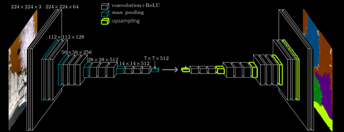
However, as mentioned previously, going from a low resolution (here 7×7) to a high resolution (224×224) is not optimal because we will lose information. That is why other architectures such as U-Net were developed:

This architecture, like FCN-16 or FCN-8, use lower stages’ output to increase the precision of the global output.
The next sections will explain how to build such models (FCN-8 on VGG-16 and U-Net) and how to train them.
2) FCN-8
2-1) Reuse feature extractor from pretrained object detection model
The last two article explained how to build an object detector, then, how to turn it into a multi-object tracker. This model was based on the famous architecture VGG-16, used as feature extractor. As the model was trained to recognize 20 classes from VOC2012 dataset, the feature extractor was trained to find good representation of these classes. As we got good results, we can use transfer learning to build a new VGG-16 model, load the weights from our object detector, then add to the VGG-16 model a module that will allow it to create segmentation maps.
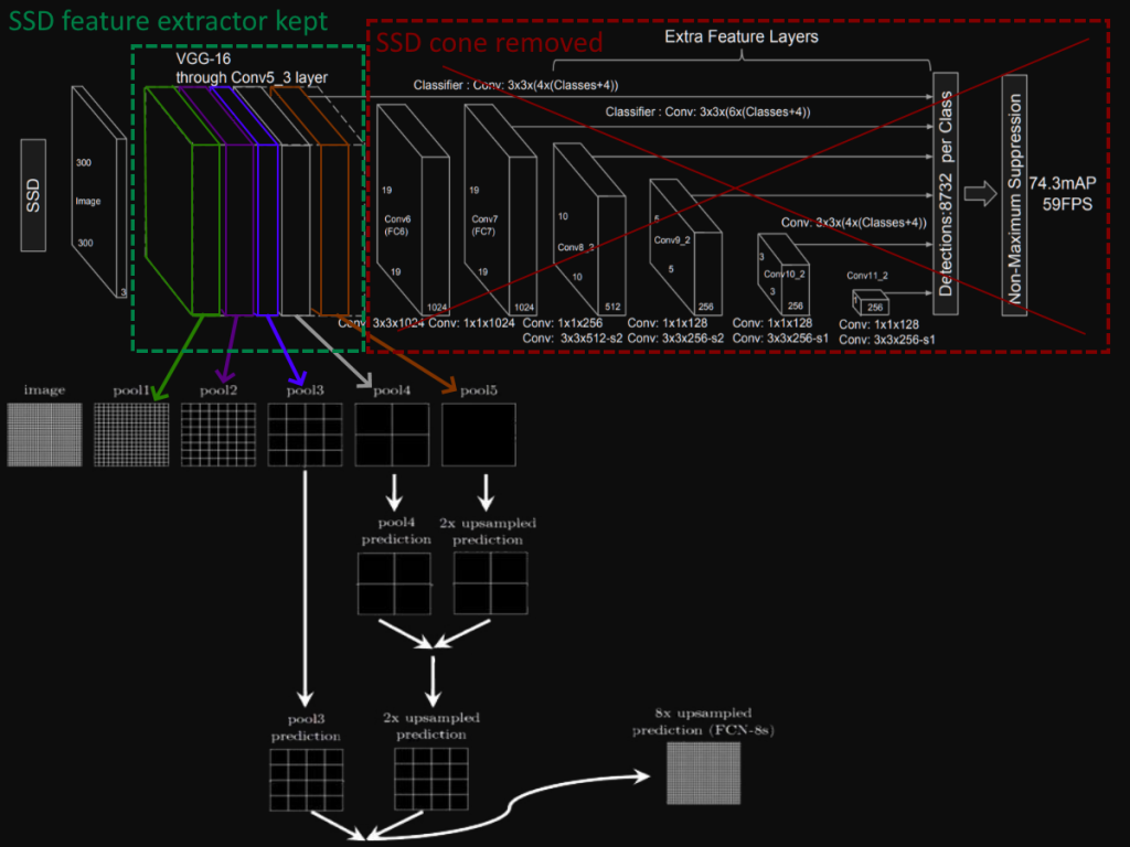
We can use several types of module to convert the output of VGG-16 to a segmentation map with resolution equals to (input width, input height, number of channels). These modules are called FCN-32, FCN-16 and FCN-8. The following illustration could help visualize what we are going to do:
- Load SSD model with weights trained on VOC2012 dataset for object detection (at this point, the feature extractor call VGG-16 learned good representation of the classes contained in VOC2012)
- Remove the “cone” of the SSD model, which is the part used for classification and regression of the bounding boxes (please refer to the previous article about SDD300 implementation to learn more about it)
- Choose the module to use: FCN-32, FCN-16 or FCN-8. For instance, to implement the FCN-8, we need to take the output of the blocks 3-4-5 from VGG-16 and apply the transformations noted (some up samplings, convolutions and concatenations)

In the next section, we will see in details how to reuse the feature extractor of a model and how to implement FCN-8.
2-2) Implementation
2-2-a) VGG-16
First, we need to create our SSD model, load its weights from a previous training on VOC2012, then, get its feature extractor VGG-16:
from models.SSD300 import SSD300
SSD300_model = SSD300(21, floatType)
confs, locs = SSD300_model(tf.zeros([32, 300, 300, 3], self.floatType))
SSD300_model.load_weights(ssd_weights_path)
SSD_backbone = SSD300_model.getVGG16()
We can then create a new VGG-16 model and copy the weights of the SSD_backbone:
from models.VGG16 import VGG16
self.VGG16 = VGG16(input_shape=input_shape)
self.VGG16_tilStage5 = self.VGG16.getUntilStage5()

for i in range(len(self.VGG16_tilStage5.layers)):
    self.VGG16_tilStage5.get_layer(index=i).set_weights(
        SSD_backbone.get_layer(index=ssd_seq_idx).get_layer(index=i).get_weights())
2-2-b) FCN-8
The following illustration shows what we are creating:
We created our VGG-16 feature extractor in the previous section. We know need to implement the FCN-8 module. As it needs the output of the stages: 3, 4, 5, we should save them to dedicated variables. If we display the VGG-16 architecture, we can know the layer indexes of each block output:
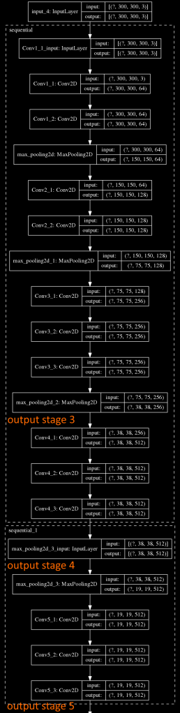
We can see in the VGG-16’s summary that the outputs we need are on indexes: 10, 14 and last one (with an additional max pooling operation):
self.inputs = tf.keras.layers.Input(shape=input_shape) # shape (300, 300, 3)
self.x = self.VGG16_tilStage5.get_layer(index=0)(self.inputs)
for i in range(1, 10):
    self.x = self.VGG16_tilStage5.get_layer(index=i)(self.x)
self.out_stage_3 = self.x

for i in range(10, 14):
    self.x = self.VGG16_tilStage5.get_layer(index=i)(self.x)
self.out_stage_4 = self.x

for i in range(14, len(self.VGG16_tilStage5.layers)):
    self.x = self.VGG16_tilStage5.get_layer(index=i)(self.x)

self.x = tf.keras.layers.MaxPool2D(
    pool_size=(2, 2), strides=(2, 2), padding='same')(self.x) # shape (10, 10, 512)
According to the FCN-8 schema, we first need to upscale x2 the stage 5 output, then concatenate it with the output of the stage 4. However, even if the resolution will be equal in width/height, we won’t have the same number of channel. As seen in the first section, a segmentation model output has (number of classes +1) channels because each feature map corresponds to a specific category + the background class. That is why we add a convolution 1×1 on the stage 4 output, to convert the number of feature maps to number of classes + 1:
# upscale x2
self.x = tf.keras.layers.Conv2DTranspose(
    n_classes, kernel_size=(4, 4),
    strides=(2, 2), use_bias=False)(self.x) # (10, 10, 512) to (22, 22, 21), 21 because there is 20 classes in VOC2012 dataset

# Cropping the resolution to match the stage 4 output resolution
self.x = tf.keras.layers.Cropping2D(
    cropping=((2, 1), (1, 2)))(self.x) # (22, 22, 21) to (19, 19, 21)

# convert the number of channels to have 1 channel per category (+1 for background)
self.out_stage_4_resized = tf.keras.layers.Conv2D(
    n_classes, (1, 1), activation='relu',
    padding='same')(self.out_stage_4) # shape (19, 19, 512) to (19, 19, 21)

# Concatenate both
self.x = tf.keras.layers.Add()([self.x, self.out_stage_4_resized])
We can then do the same logic for this input and the stage 3 output:
# upscale x2
self.x = tf.keras.layers.Conv2DTranspose(
    n_classes, kernel_size=(4, 4), strides=(2, 2),
    use_bias=False)(self.x) # (19, 19, 21) to (40, 40, 21)

# Cropping the resolution to match the stage 4 output resolution
self.x = tf.keras.layers.Cropping2D(cropping=(1, 1))(self.x) # (40, 40, 21) to (38, 38, 21)

# convert the number of channels to have 1 channel per category (+1 for background)
self.out_stage_3_resized = tf.keras.layers.Conv2D(
    n_classes, (1, 1), activation='relu',
    padding='same')(self.out_stage_3) # shape (38, 38, 256) to (38, 38, 21)

# Concatenate both
self.x = tf.keras.layers.Add()([self.x, self.out_stage_3_resized])
Finally, we can upscale x8 as we implement FCN-8:
# upscale x8
self.x = tf.keras.layers.Conv2DTranspose(
    n_classes, kernel_size=(8, 8), strides=(8, 8),
    use_bias=False)(self.x) # (38, 38, 21) to (304, 304, 21)
self.x = tf.keras.layers.Cropping2D(cropping=(2, 2))(self.x) # (304, 304, 21) to (300, 300, 21)

self.outputs = tf.keras.layers.Activation('softmax')(self.x)
self.model = tf.keras.Model(inputs=self.inputs, outputs=self.outputs)
FCN-8 is now implemented, our output shape is (300, 300, 21) which is equal to (input width, input height, number of classes +1). We can now move forward on the U-Net implementation to compare their architecture. Then, we will explain how to parse ground truth data to train these network.
3) U-Net
As mentioned in the first section, U-Net is an encoder-decoder architecture. Indeed, it reduces de width/height of the input image with 4 max pooling 2×2 (a downscale x16), then, a decoder part upscales it to retrieve the initial input resolution (the need of having the same resolution was explained in the previous section for FCN-8 implementation):
This downscaling process composes the encoder part, the network tries to reduce the complexity of the input by learning a good data representation with a downscaling x16. Then, the decoder part upscales x16 to obtain an output size equivalent to the input size. In addition to this encoding-decoding process, the architecture also use layers at different stages from the encoder part and concatenate them with the corresponding stages in the decoder part (gray arrow in the illustration). This, like for FCN-8, allows to have a better accuracy because we not only upscale data x16, we also use data from the encoder that we only upscale x8 for stage 4, x4 for stage 3, x2 stage 2, x1 for stage 1. This avoid having a low precision due to only one upscale x16.
The following code implements the encoder part. As each block looks the same except for the number of channels, we can declare them with a loop to reduce the number of lines. We can see 4 blocks with respectively 64, 128, 256, 512 number of channels for the convolutions:
# encoder part
n_filters_list = [64, 128, 256, 512]</code> # number of channels for each block
intermediate_outputs = []

for n_filters in n_filters_list:
    self.x = tf.keras.layers.Conv2D(
        n_filters, (3, 3), activation='relu', padding='same')(self.x)
    self.x = tf.keras.layers.Conv2D(
        n_filters, (3, 3), activation='relu', padding='same')(self.x)
    # save intermediate layers' output for the decoder part
    intermediate_outputs.append(self.x)
    self.x = tf.keras.layers.MaxPool2D(
        pool_size=(2, 2), strides=(2, 2), padding='same')(self.x)
    self.x = tf.keras.layers.Dropout(0.3)(self.x)
We can then add the bottleneck part:
# bottleneck
self.x = tf.keras.layers.Conv2D(1024, (3, 3), activation='relu', padding='same')(self.x)
self.x = tf.keras.layers.Conv2D(1024, (3, 3), activation='relu', padding='same')(self.x)
We now can add the decoder part which involves upscaling x2 and concatenation with intermediate outputs from the encoder part (saved in the “intermediate_outputs” list):
# decoder part
for idx, n_filters in enumerate(reversed(n_filters_list)):
    self.x = tf.keras.layers.Conv2DTranspose(n_filters, (3, 3), strides=(2, 2), activation='relu', padding='same')(self.x)
    # concatenate with intermediate encoder outputs
    self.x = tf.keras.layers.concatenate([self.x, intermediate_outputs[len(intermediate_outputs)-idx-1]])
    self.x = tf.keras.layers.Dropout(0.3)(self.x)
    self.x = tf.keras.layers.Conv2D(n_filters, (3, 3), activation='relu', padding='same')(self.x)
    self.x = tf.keras.layers.Conv2D(n_filters, (3, 3), activation='relu', padding='same')(self.x)
Finally, we can add the final 1×1 convolution used to convert the number of channels from 64 to the number of classes (the usefulness of having a number of output channels equal to the number of classes was explained in the previous section). We should also use the softmax activation function to convert the values into probabilities (for more details see previous articles) and build the model:
self.outputs = tf.keras.layers.Conv2D(
    n_classes, (1, 1), activation='softmax', padding='same')(self.x)
self.model = tf.keras.Model(inputs=self.inputs, outputs=self.outputs)
The next part will show how to build our dataset and how to train VGG-16+FCN-8 and UNet models.
4) Training
4-1) Create the dataset
As explained in the first section that about image segmentation and what is needed to train models, our ground truth data are images with labels. These image have only one channel and each pixel has a particular value depending on the category. For instance, if we have a dataset to segment cars on images, each pixel that composes a car should have the value 1, otherwise 0 (the background class). We could also have 255 values that correspond to the unlabeled pixels but we can safely replace them with 0 to be considered as background pixels.
However, as we saw in previous implementation sections, our models output images with resolution (width, height, number of classes +1), so we need the same kind of resolution for our ground truth. That is why we will create, for each ground truth image, a zero tensor of shape (input width, input height, number of classes + 1). Then, if we have 2 classes: person and dog, we will put 1 for all the pixel of the 1st channel that compose the person, we will also set to 1 all pixel of the 2nd channel that compose the dog (same for the background for the channel 0).
As a simple example we can consider the following ground truth of size 8×5 with 2 classes + the background (0):
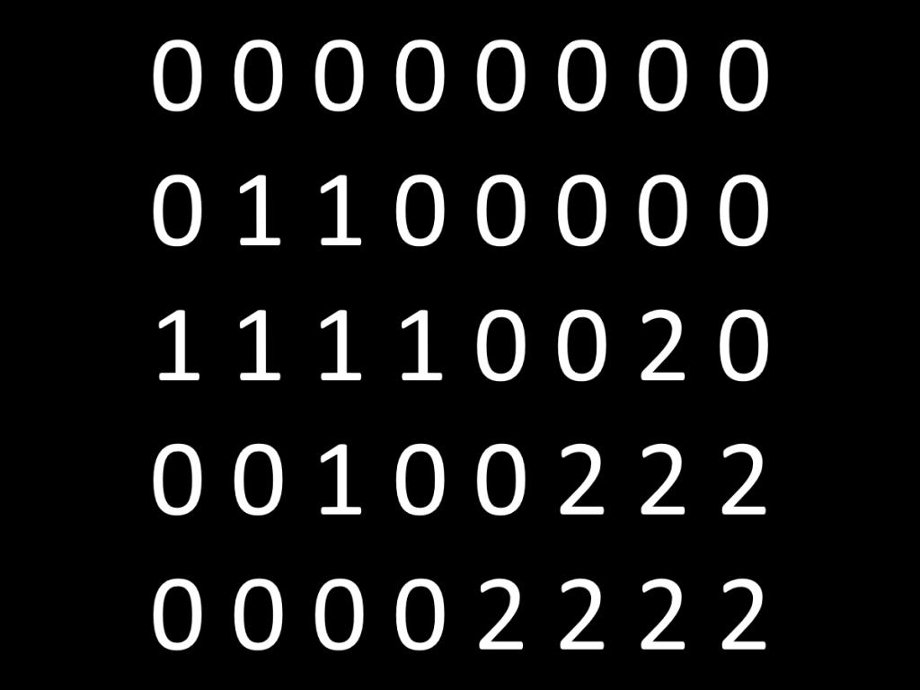
We need to create a new image of same width/height resolution but 3 channels. Each channel will have its pixel set to 1 if the corresponding class of the pixel is equal to the channel number. This will create the following three channels with the red numbers (channel 0: all background pixel set to 1, channel 1: all label 1 set to 1, channel 2: all label 2 set to 1, all the other set to 0):

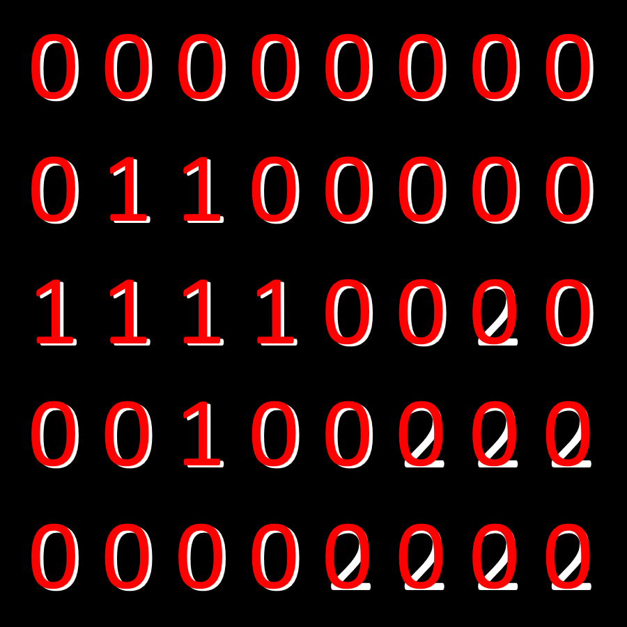

Our model can now compare its predictions (probabilities of range 0-1) with this data because each channel will have the target value 1 for the pixel of the corresponding category. The target values will be 0 for all the other pixels. The implementation for doing this conversion is not complex:
gt_annotations = []
print("Reshape gt from (width, height, 1) to (width, height, n_classes)")
for n, annotation in enumerate(tqdm(annotations)):
    stack_list = []
    # Reshape segmentation masks
    for i in range(n_classes):
        mask = tf.equal(annotation[:, :, 0],
                        tf.constant(i, dtype=tf.int16))
        stack_list.append(tf.cast(mask, dtype=tf.int16))
gt = tf.stack(stack_list, axis=2)
gt_annotations.append(gt)
The gt_annotations list will contain all our ground truth. For the input images, we only need to convert them to the input resolution and normalize them.
4-2) Compile and train the model
Contrary to the previous article, we are going to use built-in methods from tf.keras.Model: compile, ModelCheckpoint and fit.
We will first define our optimizer, then, compile le model with it:
sgd = tf.keras.optimizers.SGD(lr=0.01, momentum=0.9, nesterov=True)

model.compile(loss='categorical_crossentropy',
              optimizer=sgd,
              metrics=['accuracy'])
Contrary to the previous article where we defined a custom loss function and a custom training loop with tf.GradientTape(), we will use here .fit() method to train the model, and use ModelCheckPoint() to save the best model:. These two articles now cover both possible strategy, the use of built-in methods when possible and the use of custom loss/training function when need:
model_checkpoint_callback = tf.keras.callbacks.ModelCheckpoint(
     filepath=checkpoint_filepath,
     monitor='val_accuracy',
     mode='max',
     save_best_only=True)

history = model.fit(train_dataset, steps_per_epoch=steps_per_epoch,
                    validation_data=val_dataset, validation_steps=validation_steps,
                    epochs=epochs, callbacks=[model_checkpoint_callback])
5) Results
5-1) FCN-8; comparison with/without transfer learning from SSD model from previous article
5-1-a) With transfer learning
With transfer learning, we should expect a faster training. Indeed, the weights of the feature extractor are already trained on the target classes, so the model will only need to train the weights of the FCN-8 module to reach good scores. The following image is the first epochs of training:
We can see that our accuracy goes to 77.50% at the end of the second epoch, which very fast! After 100 epochs, we got 95.54% accuracy on the validation set:
5-1-b) Without transfer learning
Without transfer learning, all the weights are randomly initialized so the training should take longer to get the same accuracy we got on the epoch 2:
Here, our accuracy started at 35.18% and take longer to increase. We needed to wait until the epoch 19 to get a better accuracy than we got on the 2 epoch with transfer learning:

After 100 epochs, we expected to get similar results between the two models (with and without transfer learning) because the training of the model with transfer learning reaches its maximum at ~80 epochs. However, we only got 81.74% of accuracy, a huge gap!
We would need to run many more epoch to get similar results, even if the one with transfer learning got 95.19% on the 84th epoch.
5-1-c) Test on real videos
Examples of how to use functions to infer models on .mp4 videos are available on my Github profile. The following illustrations are the results I got after a person/dog training on the VOC2012 dataset (I limited the training to these two classes due to my GPU resources limitation):

The pixels classifications are good but we can notice that the segmentation map has a low resolution: made by big squares which leads to big “stairs”. This is due to the fact that the highest resolution taken from VGG-16 are of resolution 38×38 (stage 3). To fix this issue, I tried another implementation I will call FCN-4 which takes the stage 2 output of resolution 75×75 to increase the segmentation map resolution.
5-2) FCN-4
First of all, I will share an illustration of the architecture built. I won’t explain the code because it is very similar to FCN-8, there is only one more step to take the output of the stage 2 (the code is available on my Github profile under models/ folder):

With FCN-8, 95.54% of accuracy was reached after 100 epochs, with FCN-4, we got 97.15%:


The use of the stage 2 of VGG-16 fixed the issue of a low segmentation map resolution. The following illustration is a comparison between both FCN-8 (left image) and FCN-4 (right image) where we can notice the improvement in term of segmentation map resolution:


5-3) U-Net training and results
First, the input resolution was set to 128×128 to reduce the computational needs. However, even with this low input resolution, we can get good results after our training on person/dog dataset. Indeed, our dataset parser implemented in section 4 is generic enough to work with any segmentation model, we simply need to set the input resolution argument.
Contrary to the FCN-8 module that gets its maximum precision from stage 3 of VGG-16 of size 38×38 in our case, U-Net concatenates each stage of the encoder with the decoder. This means that we can get our precision increased by feature maps with resolutions 128×128 and 64×64. The “stairs” we can notice on the results with FCN-8 should be less visible with U-Net.
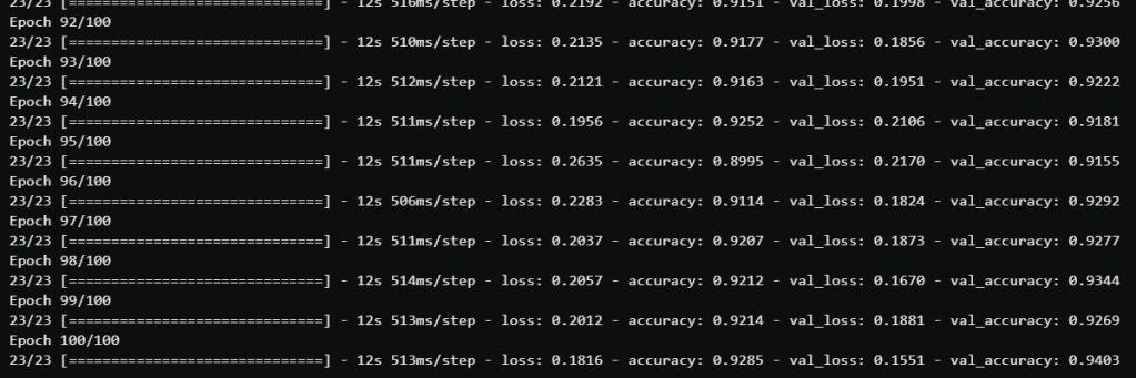
After 100 epochs, we got 94% accuracy on the validation set:
On the following animation, we can notice that U-Net is much more precise in term of segmentation map resolution. We do not have the “stairs” visible with FCN-8 anymore:

Conclusion
In this article, we learned the principle of image segmentation and how to build two types of segmentation models. The first one uses an FCN-X module that can be added to a famous feature extractor architecture. The second one, U-Net, was implemented on an encoder-decoder principle with skip connections from the encoder stages to the corresponding decoder stages. We also learned how to parse data to train our models. I hope this article will help those who want to learn more about this field.
Here you can find my project:
https://github.com/Apiquet/Segmentation
Video source: coveer

I merely found your blog and I’m immediately interested! Your content is amazing.
LikeLiked by 1 person